PaperReviews
Contents
Moving Gradients
Reproduction
- Data term: Implemented for 1-D image with exahustive search
- Regularization term
- minimization
Section 4.2.1: Assigning flows to the occluded Pixels
"So far we have only identified the occluded regions. We still need to assign flows to them for interpolation. We assume that the occluded region has one of the two flows responsible for occlusion, the fore- ground (alphabets, vB = 4) or the background (numbers, vB = 0)."
"We also assume that the occluded region as a whole is consistent
and takes the flow which majority of pixels want to take.
To determine whether the occluded region is part of the foreground
or background, we match pixel intensities, assuming that back-
ground pixels will match more closely with the background. Our
method is robust, since we match the whole area together, rather
than individual pixels separately."
This is quite vague, here are some draft ideas about how to implement it:
- identify connected components in occluded regions
- for each occluded blob, traverse each pixel and:
- look for similar pixels in foreground and background
- add to fore or back count
- if fore count > back count assign pixel to foreground
From Sparse Solutions of Systems of Equations to Sparse Modeling of Signal and Images
Lemma 1
Satatement:
For any matrix  , the following relation holds:
Proof:
First, construct a new matrix  , by normalizing the columns of
  to have unit norm
  .
This operation preserves the spark and the mutual coherence.
.
This operation preserves the spark and the mutual coherence.
Next consider the Gram matrix  . It satisfies the following properties:
- note that each entry i,j of
 is obtained by making the inner product
  . Thus
  and
and 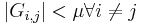
- It is semi-definite positive
- It is definite positive if and only if the columns of are linearly independent.
- The above result holds for any minor
 of size
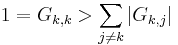
  . is definitive positive if and only if A has p L.I. columns. (3)
Next we will construct the proof with the following statements:
- Recall the Gershgorin theorem, which tells us that every eigenvalue of lies on a ball of center and radius
 .
. - If is diagonal dominant, Gershgorin's theorem guarantees us that all eigenvalues are strictly positive and thus
is positive definite and thus by (3), A has p L.I. columns.
- To let be diagonal dominant, we need the following inequality to hold:
 (1)
(1)
- As each entry
 is bounded by the coherence, if we require that
  (2)
(2)
then inequality (1) holds.
- We can rewrite (2) as:
 .
.
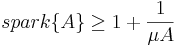
Summarizing the above results, If holds, then A has P L.I. columns. (4)
Now lets turn our attention to the spark:
- If the matrix A has spark=T, then A has T LD columns, thus T has to be greater or equal than
 , otherwise inequality (4) tells us that A must have T LI columns, which is a contradiction.
Sección 2.2.2 Convex relaxation techniques
- ademas, habria que ver la equivalencia de ambas soluciones, esto se puede ver en este artículo:
- link: D. Donoho, "For Most Large Underdetermined Systems of Linear Equations the Minimal 1-norm Solution is also the Sparsest Solution", Communications on pure and applied mathematics, Volume 59, 2006
- abstract:
We consider linear equations y = Φα where y is a given vector in Rn , Φ is a given n by m matrix with n < m ≤ An, and we wish to solve for α ∈ Rm . We suppose that the columns of Φ are normalized to unit 2 norm 1 and we place uniform measure on such Φ. We prove the existence of ρ = ρ(A) so that for large n, and for all Φ’s except a negligible fraction, the following property holds: For every y having a representation y = Φα0 by a coefficient vector α0 ∈ Rm with fewer than ρ · n nonzeros, the solution α1 of the 1 minimization problem min x 1 subject to Φα = y is unique and equal to α0 .
- quedaba en duda la afirmación de que P1 definido como abajo se podia convertir en un problema de programación lineal.
 creo que es equivalente, tomando y=Wx con W invertible, a resolver:
Sea
creo que es equivalente, tomando y=Wx con W invertible, a resolver:
Sea 
- además, también faltaba ver porque habia que normalizar cada coeficiente con la norma l-2 de las columnas de a.
Se recomienda ver el ejemplo siguiente:
Sea

y

Guigues
<graphviz caption='dubte' alt='phylogenetic tree' format='svg+png'> graph G6 { orientation=landscape node [shape=oval]; A ; B ;
C ;
D; E; F; A--B
B--C
C--E D--E E--F } </graphviz>
A la proposició 1: diu el següent: "One then always finds two edges connecting C1 and C2\C1."
Jo estic assumint que un cocoon es un subgraf connex, però no té perquè ser complet i en principi tampoc té perquè tenir cicles. Llavors et pots crear un graf com el de la figura amb dos cocoons C1={A,B,C} i C2={C,D,E,F} i no veig perquè haurien de estar connectats amb 2 arestes. Suposo que no contará dues arestes perquè el graf es no dirigit, oi?
Amb respecte a les definicions: Una altra cosa que no entenc es que passa quan hi ha dos vèrtexs desconnectats: normalment hi han dues opcions: o es posa una aresta virtual amb pes infinit o es diu directament que l'aresta no existeix. Em sembla que fa servir la segona, perquè si fa servir la primera, solament els subgrafs complets podrien ser cocoons. LLavors no entenc d'on surt aquesta propietat de les dues arestes.
Camera model
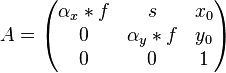
En la matriz A, f es en milimetros y \alpha es en pixels/mm. Se puede condensar todo en la matriz B, donde  es directamente en pixels.
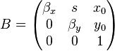 Esto está explicado en la referencia 1, páginas 5 a 8.
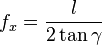 where
where  is fov/2. Thus
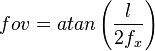
Referencias
- "Monocular Model-Based 3D Tracking of Rigid Objects: A Survey". Vincent Lepetit and Pascal Fua.
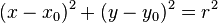
Tangente
P(x,y) en la cfa. de centro x0 y0, y radio r